While programming allows us to create virtually anything, the true test of performance arises when we deploy the same code on a significantly larger scale.
Time Complexity ($T(n)$) is a function that estimates the execution time of an algorithm given the amount of data to be processed as its input. It is a common benchmark used to measure an algorithm’s performance.
Bounds of Time Complexity
The output of the time complexity function will be a close estimate of an algorithm’s runtime yet it does not consider other characteristics of the data that could affect runtime.
Some algorithms perform best when the input data is sorted in ascending order and worst when sorted in descending order. That’s why we have bounds on the time complexity function, a range starting from best-case to worst-case execution time for the same amount of input data.
Upper Bound ($O$)
The “big O” ($O$) represents the upper bound (worst case scenario) on the time complexity function i.e. for an input dataset of size $n$ the algorithm’s time complexity couldn’t be worse than $O(n)$.
Lower Bound ($\Omega$)
The “big Omega” ($\Omega$) represents the lower bound (best case scenario) on the time complexity function i.e. for an input dataset of size $n$ the algorithm’s time complexity couldn’t be better than $\Omega(n)$.
Expected Case ($\Theta$)
The “big Theta” ($\Theta$) represents the case where both upper and lower bounds are at the same point (expected case scenario) i.e. for an input dataset of size $n$ the algorithm’s time complexity couldn’t get better or worse than $\Theta(n)$.
Big $O$ is the preferred time complexity function for an algorithm’s runtime analysis because it provides a conservative estimate and its result is independent of factors like hardware performance, characteristics of data, compiler optimization, etc.
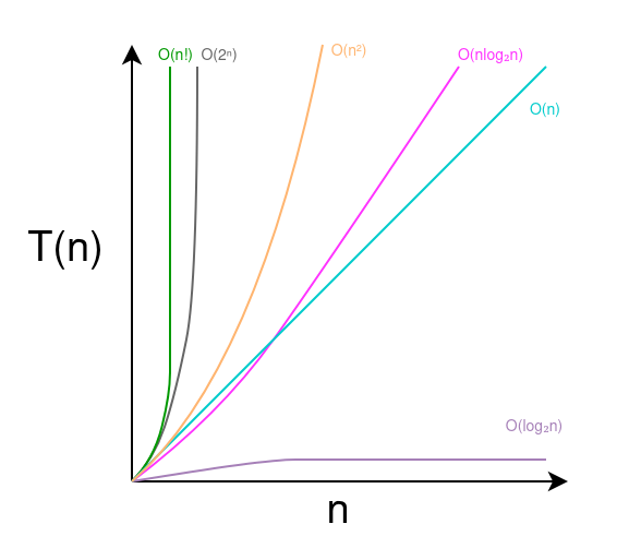
Common Time Complexity Functions
The runtime of recurring patterns in programming could be represented by common time complexity functions. This helps us estimate the time complexity of the entire program.
Constant Time Complexity $O(1)$
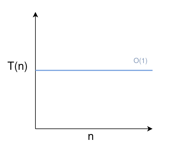
Scaling an Algorithm with Constant Time Complexity
An algorithm has constant time complexity when its runtime isn’t affected by the amount of data passed as input. An example would be a function that performs addition on its two inputs.
package main

import "fmt"

func addition(x int, y int) (int){
	// The size of x and y does not affect
	// the runtime of this function

	return x+y
}

func main(){
	x := 2000
	y := 2132
	fmt.Println("Addition of", x, "and", y, "is:", addition(x, y))
}

// Result
// Addition of 2000 and 2132 is: 4132
The above example is implemented in the Go Programming Language.
Linear Time Complexity $O(n)$
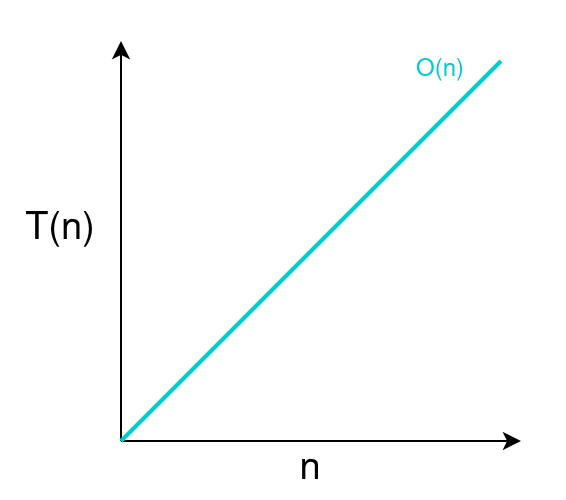
Scaling an Algorithm with Linear Time Complexity
For some algorithms the execution time is directly proportional to the size of its input, such algorithms are categorized in linear time complexity.
An example would be a loop that iterates over elements in a list and returns its sum.
package main

import "fmt"

func arraySum(arr []int)(int){
	sum := 0

	// Time taken to complete this loop
	// will be directly proportional to the
	// size of arr
	for _, element := range arr{
		sum += element
	}

	return sum
}

func main(){
	arrayExample := []int{1, 2, 3, 2, 1, 1}
	fmt.Println("Sum of the array:", arrayExample, "will be",
                arraySum(arrayExample))
}

// Output
// Sum of the array: [1 2 3 2 1 1] will be 10
If we call the function arraySum() twice then the time complexity of the program will be $O(2n)$. However, we can generalize it to $O(n)$ because even though the program performs two passes over the array, the growth rate in runtime remains linear with respect to its input size.
Quadratic Time Complexity $O(n^2)$
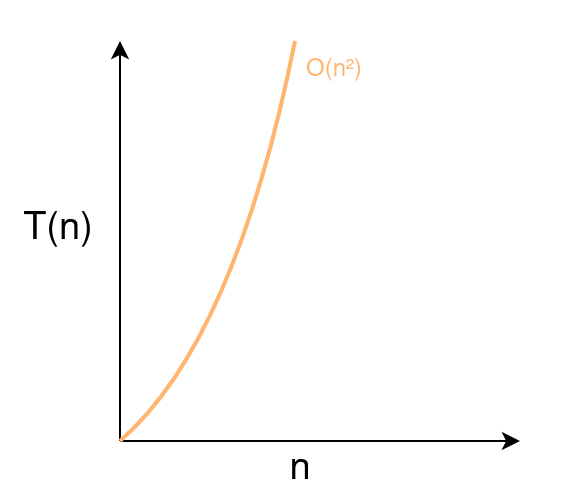
Scaling an Algorithm with Quadratic Time Complexity
Similar to linear time complexity, algorithms exhibiting quadratic time complexity experience execution times that are directly proportional to the square of the number of inputs. These algorithms scale relatively slower (longer execution time) compared to linear time complexity algorithms like $O(n)$, $O(2n)$, etc.
For example, a program that displays pair combinations of all elements in an array using nested loops.
package main

import "fmt"

func showCombinations(arr []int){

	// The inner loop is executed n (size of arr) times.
	// Thus, the total time complexity of this function will be O(n*n)
	for _, element1 := range arr{

		// Time complexity of the inner loop
		// is directly proportional to the size of arr i.e. O(n)
		for _, element2 := range arr{

			if(element1 != element2){
				fmt.Println("Combination:", element1, "and",
                                            element2)
			}

		}

	}
}

func main(){
	arrayExample := []int{123, 1234, 456, 5462}
	fmt.Println("Pair combination of all elements in the array: ",
                arrayExample, "are:")
	showCombinations(arrayExample)
}

// Output
// Pair combination of all elements in the array:  [123 1234 456 5462] are:
// Combination: 123 and 1234
// Combination: 123 and 456
// Combination: 123 and 5462
// Combination: 1234 and 123
// Combination: 1234 and 456
// Combination: 1234 and 5462
// Combination: 456 and 123
// Combination: 456 and 1234
// Combination: 456 and 5462
// Combination: 5462 and 123
// Combination: 5462 and 1234
// Combination: 5462 and 456
Exponential Time Complexity $O(2^n)$
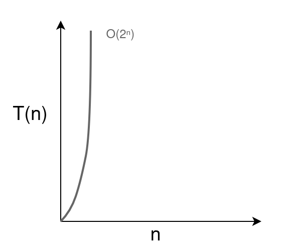
Scaling an Algorithm with Exponential Time Complexity
A brute-force algorithm to find the $n$th number in the Fibonacci series has exponential time complexity because it branches in two recursive calls on every iteration.
package main

import "fmt"

func fibonacci(n int) (int){
	if n <= 1 {
		return n
	}

	// The recursive calls will branch
	// further in two more calls
	return fibonacci(n-1) + fibonacci(n-2)
}

func main() {
	n := 10
	fmt.Println("The", n, "th Fibonacci number is:", fibonacci(n))
}

// Output
// The 10 th Fibonacci number is: 55
Algorithms with $O(2^n)$, $O(e^n)$, $O(10^n)$, etc. time complexities are grouped under exponential time. Among these, the $2^n$ function has widespread use in computer science like Moore’s law or to find the number of memory addresses possible with $n$ bits arrangement.
The number of transistors in an Integrated Circuit (IC) doubles about every two years
Gordon Moore, Co-Founder of Intel, 1965
Logarithmic Time Complexity $O(\log_2{n})$
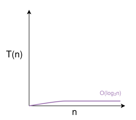
Scaling an Algorithm with Logarithmic Time Complexity
The $\log_2{n}$ is the inverse of function $2^n$. The following example of a number guessing game has $O(\log_2{n})$ time complexity because it cuts the search space by half on each iteration.
package main

import "fmt"

func guessNumber(low int, high int)(int){
	// Returns the middle number in a range from low to high
	mid := (high+low)/2
	return mid
}

func main(){
	low := 0
	high := 100
	fmt.Println("Think of a number between", low, "and", high)
	numQuestions := 0

	for {
            var answer1, answer2 int
            guessedNumber := guessNumber(low, high)

            fmt.Println("I guessed:", guessedNumber, "Is that correct?")
            fmt.Println("1) Yes")
            fmt.Println("2) No")
            fmt.Print("Enter your response (1 or 2):")
            fmt.Scan(&answer1)

            switch(answer1){
                case 1:
                    fmt.Println("It took me",
                                numQuestions,
                                "questions to guess your number")

                    // It will take maximum log(n) questions to guess a number
                    // Where n is size of the number range in this case 100

                    fmt.Println("Thanks for playing")
                    return

                case 2:
                    numQuestions += 1
                    fmt.Println("Is it higher or lower than", guessedNumber)
                    fmt.Println("1) Higher")
                    fmt.Println("2) Lower")
                    fmt.Print("Enter your response (1 or 2):")
                    fmt.Scan(&answer2)

                    switch(answer2){
                        case 1:
                            // Halving the search space
                            // to exclude number lower than guessed
                            low = guessedNumber
                        case 2:
                            // Halving the search space
                            // to exclude number higher than guessed
                            high = guessedNumber
                    }
            }
	}
}

// Output
// Think of a number between 1 and 100
// I guessed: 50 Is that correct?
// 1) Yes
// 2) No
// Enter your response (1 or 2):2
// Is it higher or lower than 50
// 1) Higher
// 2) Lower
// Enter your response (1 or 2):2
// I guessed: 24 Is that correct?
// 1) Yes
// 2) No
// Enter your response (1 or 2):2
// Is it higher or lower than 24
// 1) Higher
// 2) Lower
// Enter your response (1 or 2):1
// I guessed: 37 Is that correct?
// 1) Yes
// 2) No
// Enter your response (1 or 2):1
// It took me 2 questions to guess your number
// Thanks for playing
Linearithmic Time Complexity $O(n \log_2 n)$
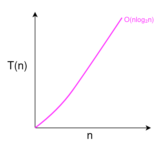
Scaling an Algorithm with Linearithmic Time Complexity
Merge Sort, Quick Sort, and Heap Sort are some examples of algorithms with linearithmic time complexity.
Factorial Time Complexity $O(n!)$
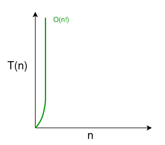
Scaling an Algorithm with Factorial Time Complexity
The solution to the Travelling Salesman Problem has factorial time complexity.
Comparing Algorithm Performance Using Time Complexity
In a hypothetical scenario, we have benchmark sorting performance of different algorithms by their time complexity.
Assuming the output of the time complexity function is the algorithm’s execution time in seconds. The runtime of a sorting algorithm on 100 elements with
- $O(\log_2{ n})$ time complexity is 6.644 seconds
- $O(n)$ time complexity is 100 seconds
- $O(n \log_2 n)$ time complexity is 664.4 seconds
- $O(n^2)$ time complexity is 10000 seconds (2.7 hours)
- $O(2^n)$ time complexity is $1.26 \times 10^{30}$ seconds ($3.99 \times 10^{22}$ years)
- $O(n!)$ time complexity is $9.33 \times 10^{157}$ seconds ($2.9585 \times 10^{150}$ years)

Time Complexity Comparison of Algorithms
With the same computation power, an algorithm with $O(2^n)$ time complexity will sort 100 elements in $3.99 \times 10^{22}$ years while an algorithm with $O(n \log_2{n})$ time complexity will take only 664.4 seconds .
Thank you for taking the time to read this blog post! If you found this content valuable and would like to stay updated with my latest posts consider subscribing to my RSS Feed.
Resources
Big Theta and Asymptotic Notation Explained
What is Moore’s Law
Relationship between exponentials & logarithms
The factorial function